Staff Engineer at Instruqt
I bet you never thought about it, as the problem seems trivial. When you drive with GPS-enabled navigation in your car, how does your smartphone/car navigation know which street you are on? You yourself mostly know it, even if you could not look outside the window, just eyeballing the route on the screen is enough to intuitively, fast, and with little uncertainty tell which road you are on right now and how you got there.
Even when the GPS jitters, jumps around, or is a bit off to the side, this is not enough to confuse a human. The GPS measurement error and sampling rate, however, combined with dense urban roads are enough to confuse a computer. In short: matching a series of GPS measurements to a known road is certainly possible, just not as easy to express in code.
Ok but why?
At Plotwise we are in the business of last-mile delivery planning, we provide optimal routing for deliveries. Once the driver receives the plan, how do we know it was actually followed? Maybe it was unrealistic or based on faulty data? Using GPS measurements from the delivery tracks is a feedback mechanism we need to validate our planning.
In general, in any non-trivial case of working with GPS measurements for vehicles, you would want a reliable way to match it to the roads.
Let's try a naive approach first and see its limitations.
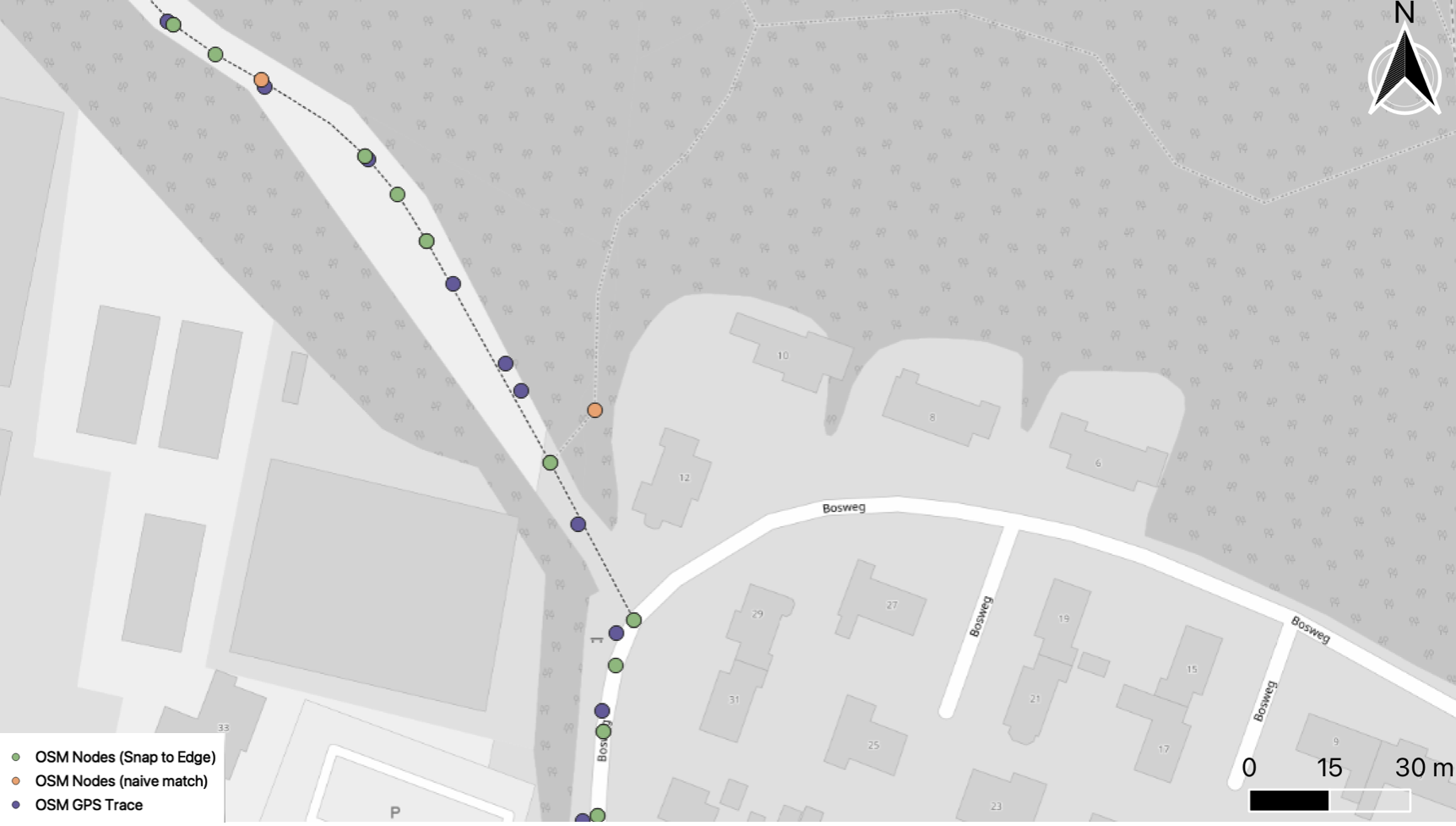
The picture below shows road nodes as known to Open Street Maps. This is a small area in the city of Assen, Drenthe, The Netherlands. I downloaded the data from the Open Street Maps GPS trace directory.
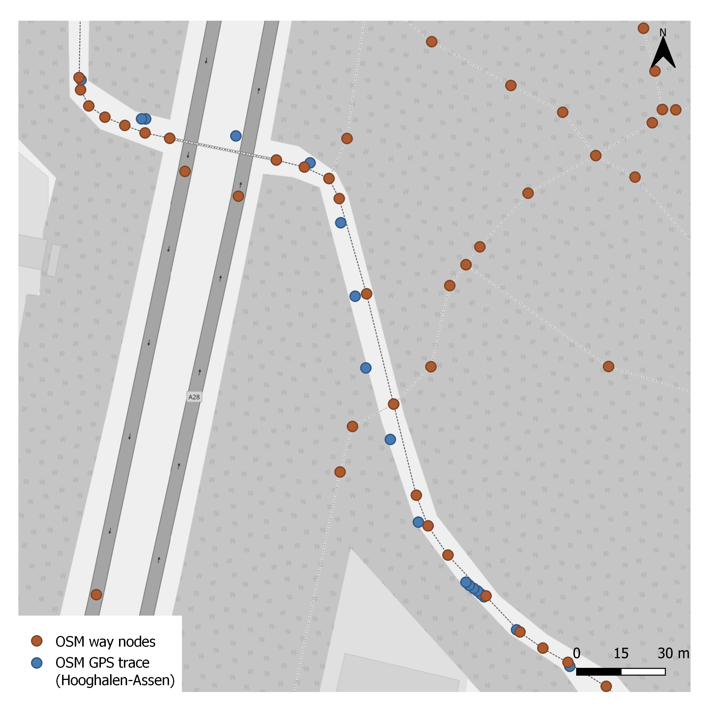 As you can see each road is represented by multiple nodes, let's call an edge between two nodes of the same road a "road segment".
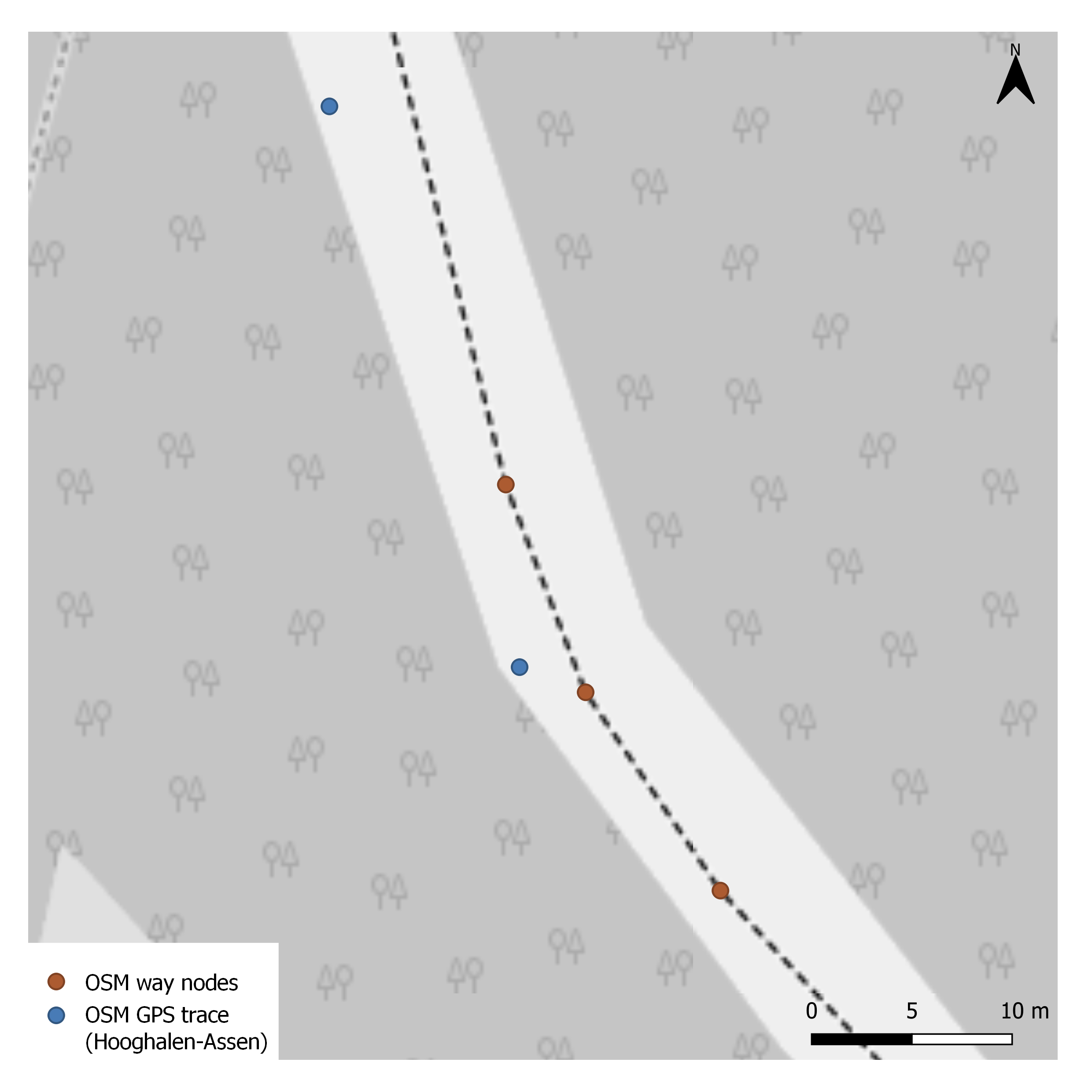 On the picture above, you see a zoomed-in view of the same area, with one road consisting of several nodes, some of them close to a GPS reading (a red node). Characteristically the GPS measurement is off to one side of the road, in this case, it is still easy to assign it to the closest road segment (although even in this case, it is no longer obvious which road node is the best match for the node in the upper section of the map).
What if we just pick the road node closest to the GPS node?
The first detail to sort out: the distance metric. My own instinct was to use a euclidean distance, but while working with latitude and longitude expressed in degrees this is plain wrong. Earth you see is not flat, so we need to use a bit of trigonometry to acknowledge this fact, otherwise the further away we get, the worse the error we generate. Because the distances between any (actually useful) GPS measurements are small, we can rely on so-called haversine distance, there is a nice python package implementing it, scipy also provides it. Once we have a distance metric sorted out, however, the naive method is straightforward and pretty much as you would expect. Have a look at a simple Python implementation of the naive GPS matching method.
def naive(gps, local_road_network: Graph) -> DiGraph:
    """Match GPS to roads using proximity.

    Given a list of ordered gps measurements and
    a graph of local roads, compute a directed graph
    of local road nodes that match by geographical
    proximity to the gps measurements.
    """
    all_nodes = local_road_network.nodes()
    estimated_path = []
    for measurement in gps:
        best = None
        best_dist = None
        for node in all_nodes:
            dist = haversine(measurement, node)
            if not best or best_dist > dist:
                best = node
                best_dist = dist
        estimated_path.append(best)
    path_graph = DiGraph()
    # construct a path from the list, n2 is the element following
    # the n1 in the sequence
    for n1, n2 in zip(estimated_path[:-1], estimated_path[1:]):
        path_graph.add_edge(n1, n2)
    return path_graph
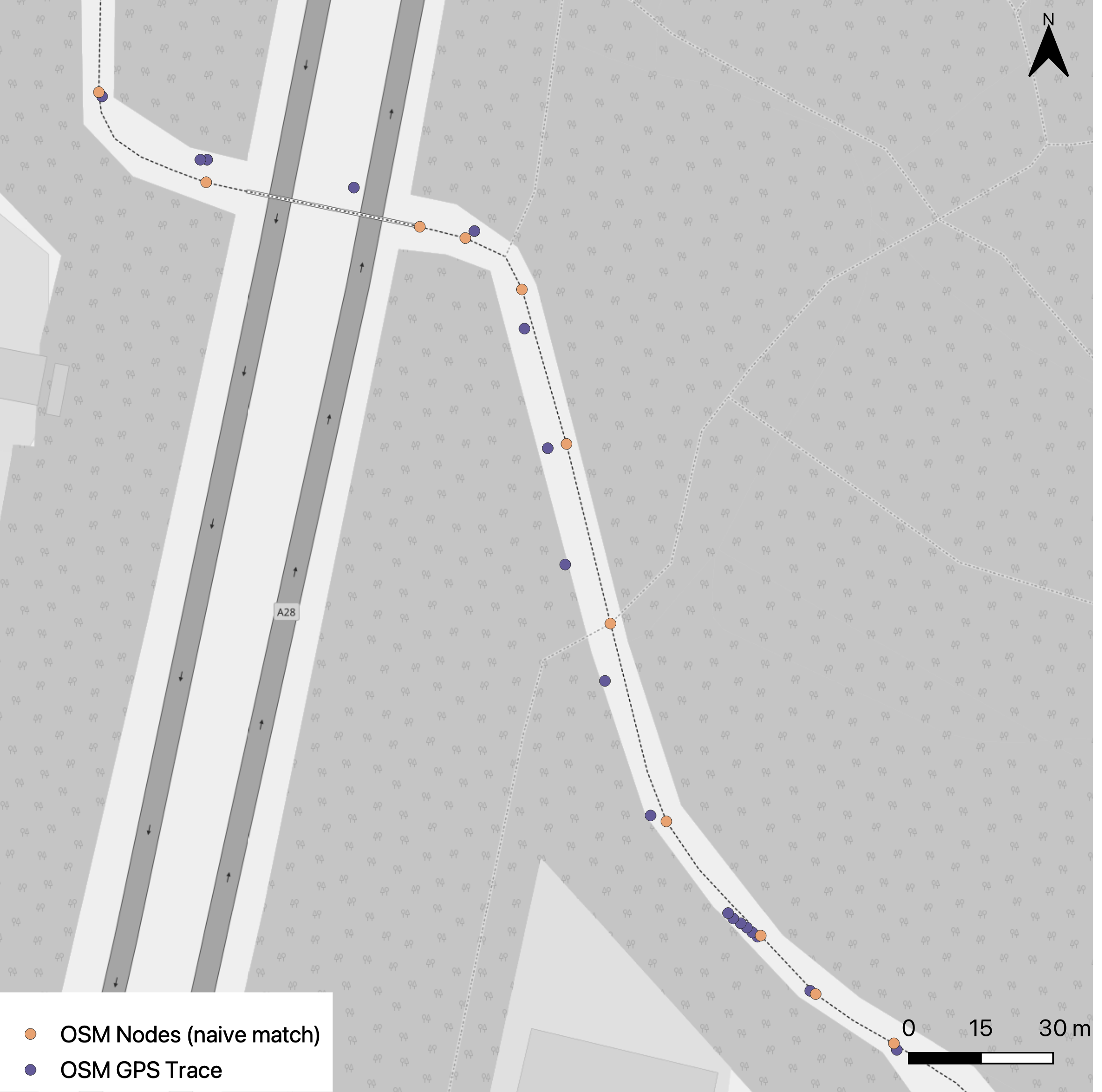
This method performs well enough on a straight road in a not too dense of an area. Have a look for yourself, below are the matching results for the naive method.
Now to a non-trivial case
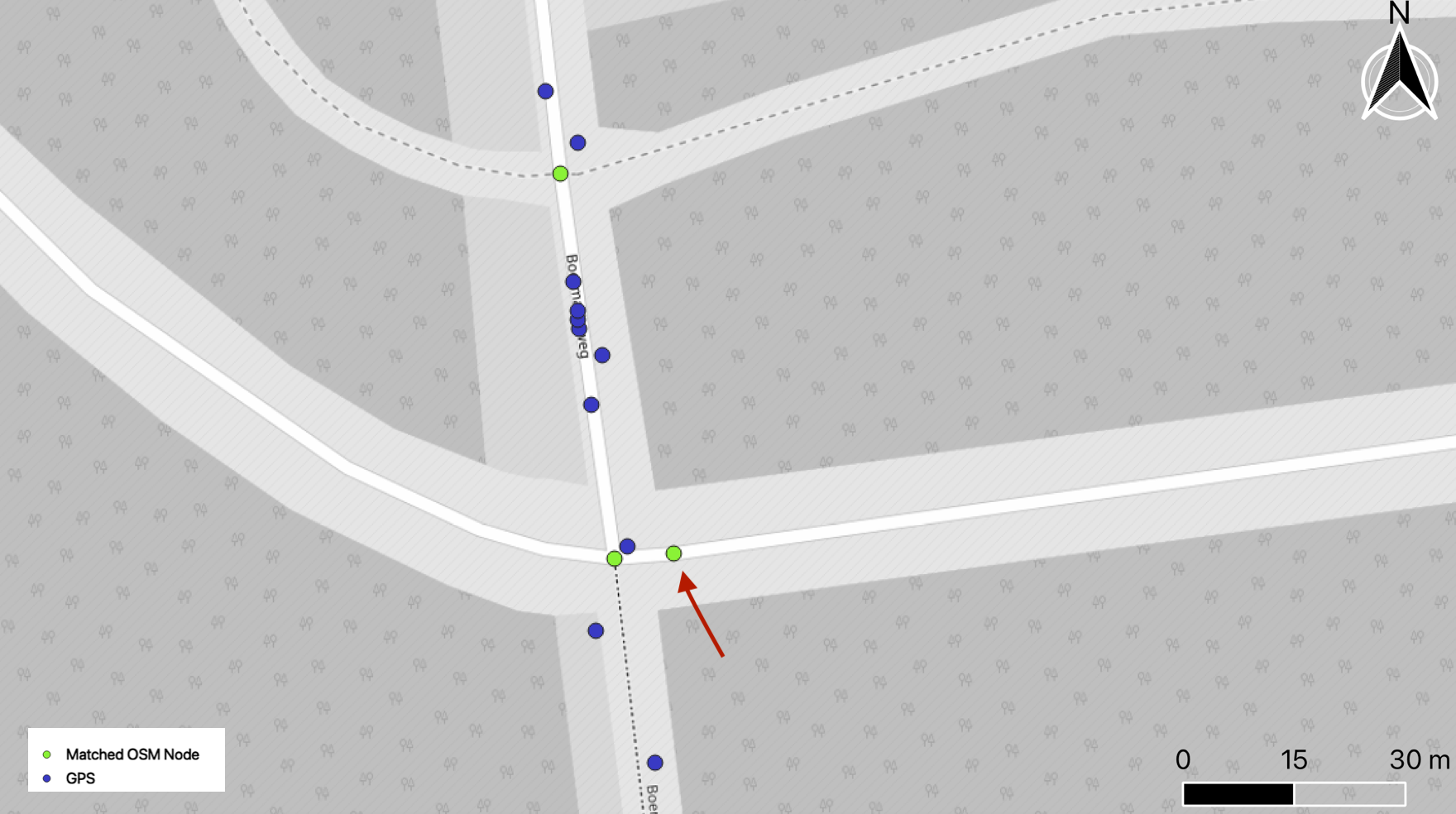
But it wouldn't be much of a blog post if the naive approach was all there is to it right? You all came here for some obscure maths and crazy algorithms, or a tool to match GPS to OSM (that will come later too). Let's consider some more complex cases, which happen in real-life situations (esp in an urban setting) all the time. In fact, we don't have to look too far as one pretty good example hidden in plain sight in the simple GPS trace from Drenthe, the Netherlands we have been looking at so far ...
This is an intersection at the bottom of the map. You can easily tell that the orange (matched) node to the right (eastern) side of the intersection is incorrect, given the GPS trace as seen on the map, you can safely assume that the biker went straight and not ... well, teleported themselves for a brief moment 15 m to the right just to continue back on the straight line as before.
Intuitive Fix
Before we try looking for anything fancy and state-of-the-art from GIS literature, let's try to improve the naive method to account for the above case. What caused this GPS reading to be matched to the perpendicular road instead of the one it clearly is on? This is an artifact of the representation of roads in my simple implementation. I calculate the distance between the OSM nodes and the nodes are points, not lines, they are also somewhat sparse, there is only enough of them to allow to draw the shape of the road precisely. It seems that using a distance from a GPS reading (a point) to a line between two consecutive OSM road nodes (points) should eliminate this silly error.
def naive_edge(gps: List[GPSMeasurement], local_road_network:Graph) -> DiGraph:
    """Match GPS to roads using proximity.

    Given a list of ordered gps measurements and
    a graph of local roads, compute a directed graph
    of local road nodes that match by geographical
    proximity of the gps measurements to a line between
    two road nodes.
    """
    all_nodes = local_road_network.nodes()
    estimated_path = []
    for measurement in gps:
        # get all road nodes within 20m of the measurement
        closest = get_in_proximity(measurement, all_nodes, 20)
        if not closest:
            print(f"loc {measurement} has no close OSM nodes")
            continue
        # start at any node within 20m
        starting_node = closest[0]
        best = None
        best_dist = None
        # conduct depth first search with max depth of 3 around the first node
        for road_node1, road_node2 in dfs_edges(local_road_network, source=starting_node, depth_limit=3):
            # snap_to_edge finds a point on the line between two points that is
            # the closest to the third point, in our case the two points
            # forming the line are some two OSM nodes and the third one
            # is the GPS measurement. See https://stackoverflow.com/questions/3120357/get-closest-point-to-a-line
            snapped = snap_to_edge(road_node1, road_node2, measurement)
            dist = haversine(measurement, snapped)
            if not best or best_dist > dist:
                best = road_node1, road_node2
                best_dist = dist
        estimated_path.append(best)
    path_graph = DiGraph()
    for n1, n2 in estimated_path:
        path_graph.add_edge(n1, n2)
    return path_graph
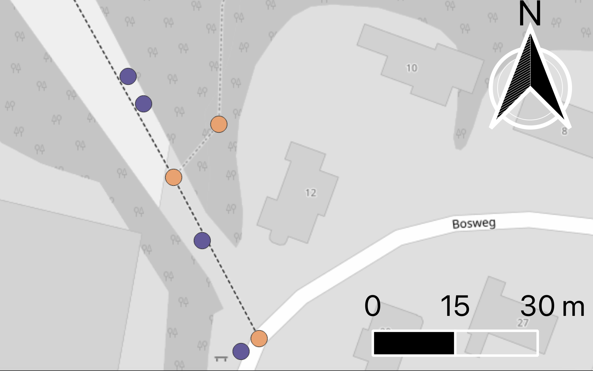
As expected, snapping to the closest edge instead of a node solves the irregularity, new method results are in green. When they overlap with the old ones, the green prevails, the old orange ones are shown only where those are NOT replicated by the new method:
Encouraged by the success of this method I ran it on a bigger GPS trace and inspected the quality against my infallible human judgment. Alas, while snapping to edge instead of node leads to better results, quite often it is still not enough. Especially at intersections.
Why is the node to the right of the bottom intersection (green) matched? Well, it really IS the closest to the GPS node even when measuring against the edge made from its osm nodes and not the OSM nodes themselves ... the edge made by the offending OSM node and the intersection node is the closest one, so it was matched by our simple algorithm.
How do I know that this is an incorrect match then? Because I imagine how the vehicle that left this trace behaved, I know that each GPS measurement took place in a brief succession and if both following and preceding nodes indicate traveling in a straight line, but the measurement in between falls just marginally to the side I will still match the measurement to the straight line. In other words, I imagine what would it take to transition from one node to another, taking into consideration more than just one GPS measurement at the time.
State-of-the-art GPS to map matching algorithms are based on Hidden-Markow-Models(HMM) these days. One of the more accessible and production-ready implementations of which is in Valhalla. Implementing an HMM-based algorithm for map matching is significantly more involved, it is material for a separate blog post, a brief intro into using Valhalla for map matching can be found in this helpful blog post. Let's use Valhalla on the same GPS trace from Drenthe and see if it manages to account for neighboring GPS measurements (a.k.a transition probability) correctly and eliminate the unrealistically matched node to the side of the crossroad.
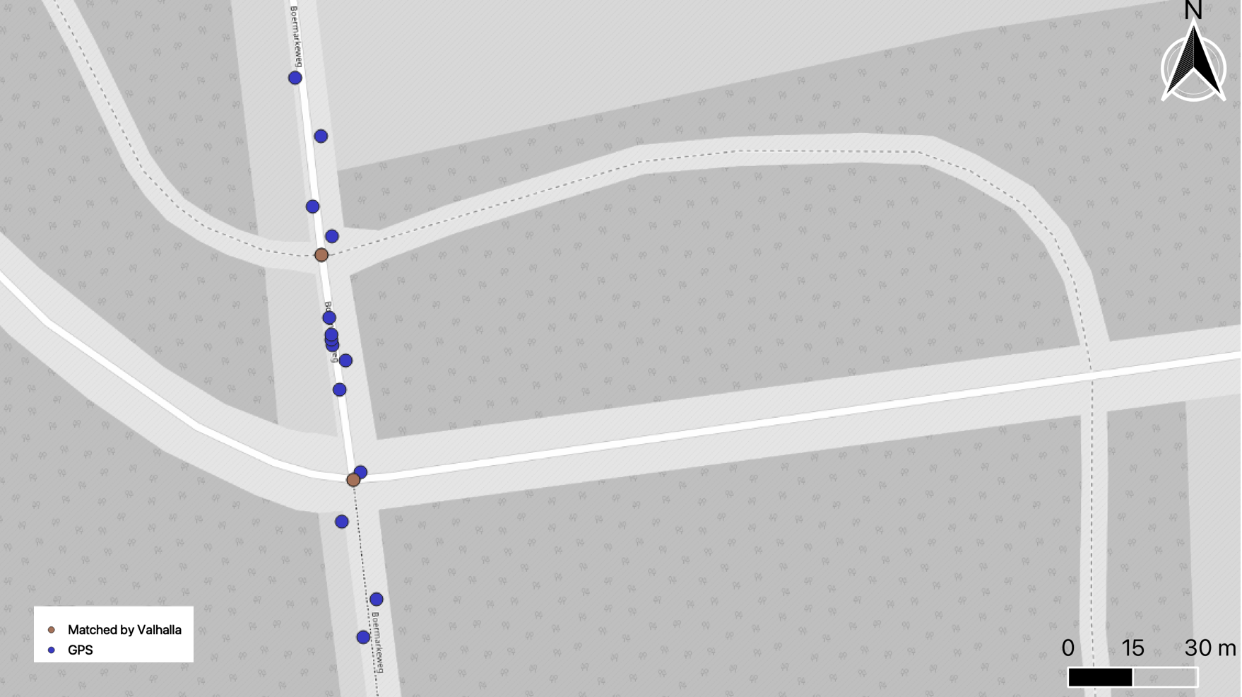
Output from Valhalla is much cleaner, does not include the node to the right side of the intersection as expected. For two reasons: first, it accounts for the possibility of such transition (it looks at more than just one GPS measurement at a time), and second ... that it reports only a minimal amount of nodes needed to make a route. It reports only the intersections in other words.
Conclusion
Matching GPS measurements is complicated by several factors:
- inherent GPS measurement error (measurements will appear some semi-random distance from your real position)
- road network density, for instance in highly urbanized areas (esp. in combination with the GPS error, it may make measurements appear closer to parallel roads and thus harder to match)
- road representation: node vs edge, but also level of detail (intersection only, or more nodes per road segment? Inclusion of bike-paths/service roads?)
- measurement frequency (it is taken at intervals), gaps between measurements need to be interpolated
The currently applied approach to the problem is based on Hidden Markow Model, which sufficiently accounts for all the above because it uses transition probability, or what a human would call "how likely that the vehicle would really travel through here given other measurements nearby".
At Plotwise we work on problems like this one to solve the last-mile delivery crisis, check out our career page if you want to join our mission